Predictive Maintenance of Forklifts using Sensor Data
Published:
Kaufland Solution – LSTM and EDM Models for Predictive Maintenance
| Posted 29.09.2018 | william ardianto, teoh kenghooi, narjes khatoon,yee xunwei, philip khor |
In this paper we propose the use of a combination of LSTM and EDM models to address the issue of anomaly classification and prediction in time series data. Working with sensor data for automated storage and retrieval systems for a German hypermarket chain, we show that predictors based on variance and median methods show sufficient promise in the handling of anomalies.
1. Business Understanding
As part of the Kaufland challenge, we are tasked to build a predictive maintenance model to avert machine failure. Internet of Things (IoT) sensors allow us to monitor the machine’s performance in real time. The model can detect when the machine performs anomalously and suggest the need for action on specific parts of the machine that is about to fail. A predictive system that can detect anomalies in the machine’s behaviour just before it breaks down will help minimise maintenance costs. Compared to a preventive maintenance system, a predictive system is able to reduce costs associated with preventive maintenance done even when maintenance is not required. The business success criteria would therefore be to lower maintenance costs relative to a preventive maintenance system.
Predictive maintenance is a strategy to reduce cost of:
- Labour for skilled repairman
- Preventative part replacement
- Post damage repair which might be higher than preventive maintenance
- Overcome the availability of experts to repair machines
The predictive system will be a success if it detects anomalies accurately.
Our project plan is summarised in Figure 1. The first step consists of exploratory data analysis and data preparation. Based on the first step, we decide on our modelling approach and then construct a strategy for deployment.
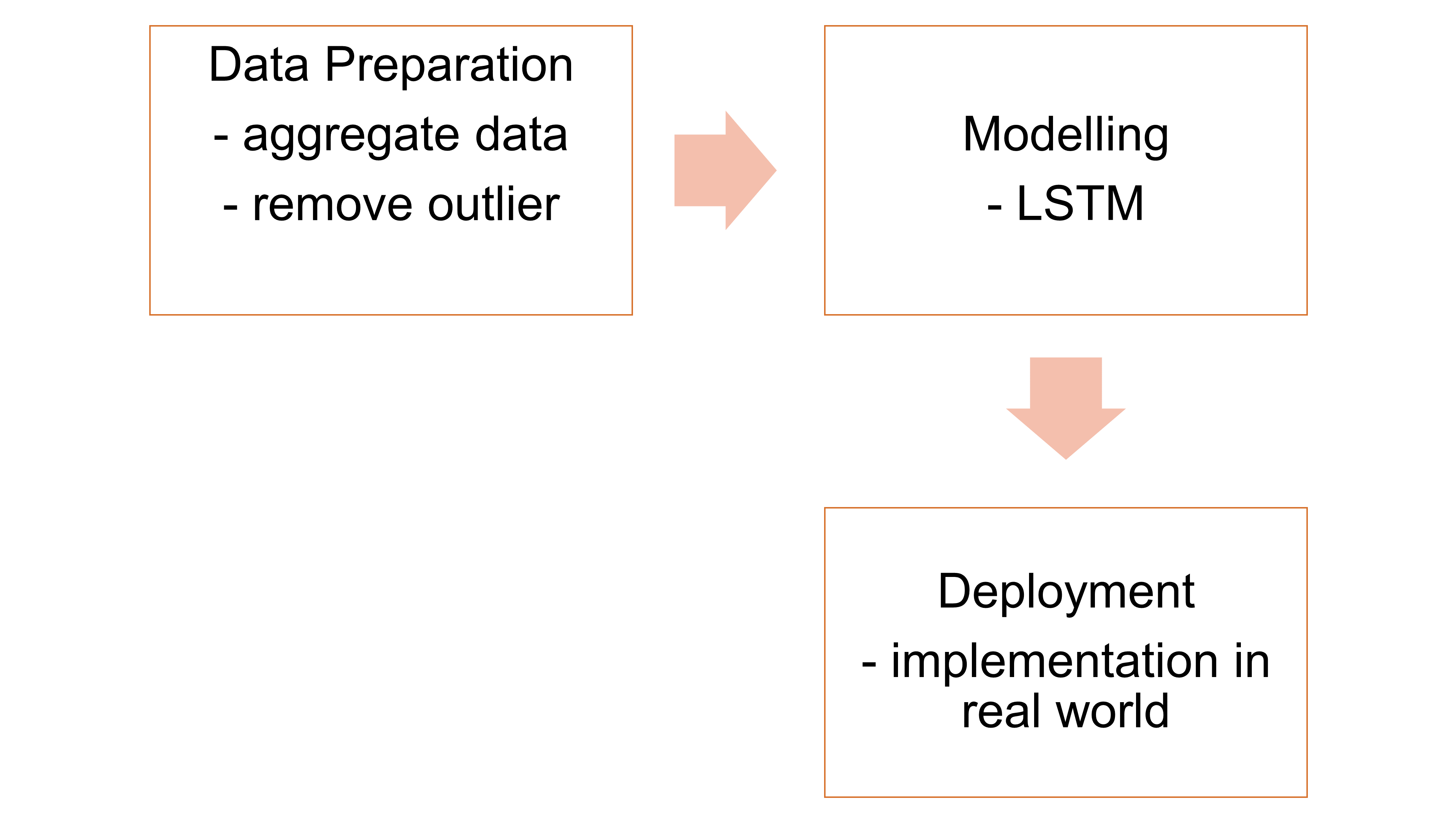
Figure 1: Project plan
In this project, we have access to a dataset of sensor data (velocity and acceleration) attached to seven machines over a period of 5 months to two years.
The tools that we consider for this purpose are Python and R, which are popular languages for statistical and data analysis. Given that our team has mixed proficiency in both languages, we conduct our analysis in a mix of both. The models that we consider for this purpose at the preliminary stage are Long-Short-Term Memory (LSTM) models.
The goal is not to determine how much vibration a machine will withstand before failure. The aim is to obtain a trend in vibration characteristics that can warn of trouble. For example a sudden short peak or increase does not necessarily means the machine is going to fail, it might be caused by sensor error. Instead, look for odd occurrence that persists.
2. Data Understanding
The data is loaded in R and Python. The data we use is provided by Kaufland, a large hypermarket chain based in Germany. We are provided with data on 7 separate automated storage and retrieval systems machines. Each machine has 6 different sensors (Figure 2). Data from these machines are collected for different time ranges:
- 2 years for Machine 1 and 7 (RBG1 and 7).
- 5 months for the other machines.
RBG 1 and 7 are the pilot study to test the efficiency of the sensors, this explains why they have long range of data. Sensors are embedded to the other machines after the sensors are proved to be working.
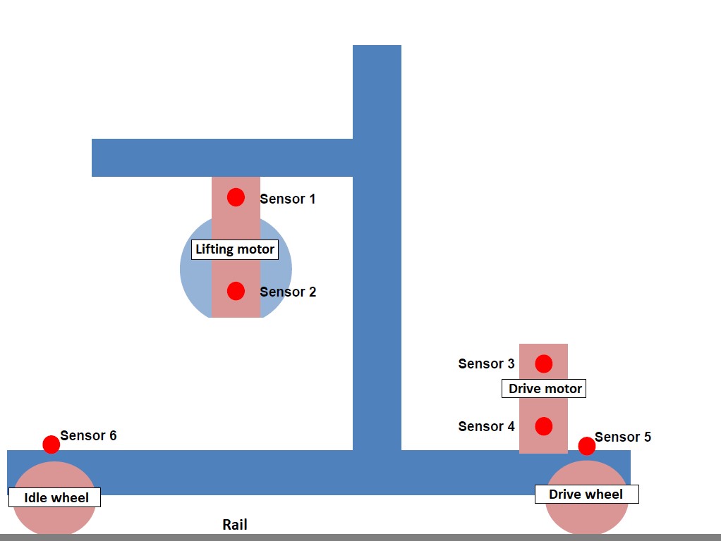
Figure 2: Sensors on machine. Image from Data Science Society.
The sensors attached to the machine are as follows:
- Lifting mechanism:
- Sensor 1: Lifting motor
- Sensor 2: Lifting gear
- Drive mechanism:
- Sensor 3: Drive motor
- Sensor 4: Drive gear
- Sensor 5: Drive wheel
- Sensor 6: Idle (non-powered) wheel
These six sensors measure the effective velocity of vibrations and the maximum acceleration of shocks, collected under controlled conditions thrice a day.
Figure 3 shows a sample of data from the drive gear sensor on Machine 1. All these sensors measure both the effective velocity of vibrations and the maximum acceleration of shocks. Each sensor collects data under controlled conditions three times a day. Two of the machines have collected data for almost two years, the other five for five months.
| machine_name | sensor_type | date_measurement | realvalue | unit | start_time | end_time | day_of_week | sensor_group | |
|---|---|---|---|---|---|---|---|---|---|
| 0 | RBG1 | drive_gear_V_eff | 2/9/2016 | 0.395 | mm/s | 26:42.8 | 26:42.8 | Friday | driving_motor |
| 1 | RBG1 | drive_gear_V_eff | 2/9/2016 | 0.577 | mm/s | 26:45.7 | 26:45.7 | Friday | driving_motor |
| 2 | RBG1 | drive_gear_V_eff | 2/9/2016 | 0.717 | mm/s | 26:48.5 | 26:48.5 | Friday | driving_motor |
| 3 | RBG1 | drive_gear_V_eff | 2/9/2016 | 0.832 | mm/s | 26:51.3 | 26:51.3 | Friday | driving_motor |
| 4 | RBG1 | drive_gear_V_eff | 2/9/2016 | 0.941 | mm/s | 26:54.1 | 26:54.1 | Friday | driving_motor |
| 5 | RBG1 | drive_gear_V_eff | 2/9/2016 | 1.042 | mm/s | 26:56.9 | 26:56.9 | Friday | driving_motor |
Figure 3: Data from drive gear sensor of Machine 1.
3. Data Exploration
Data exploration is performed with purpose of finding relationships among factors to motivate a modelling approach.
The values of vibrations of sensors for each sensor is plotted using scatter plot (Figure 4 and 5). The values of six sensors are included. Null values are not shown in the figures.
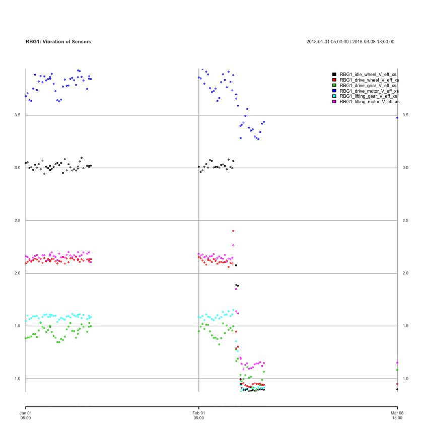
Figure 4: Values of sensors for Machine 1 (RBG1). This machine shows a significant decrease in mean vibration read after a documented maintenance event on 8 Feb 2018.
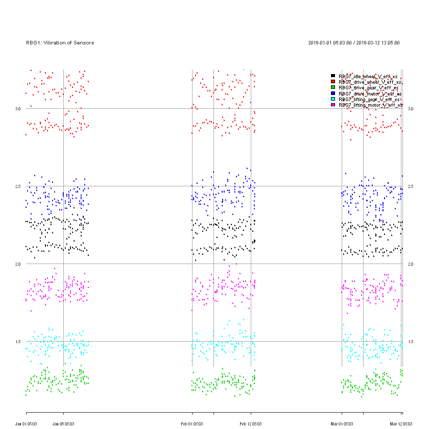
Figure 5: Values of sensors for Machine 7 (RBG7)
Correlation matrix is plotted in Figure 6. Matrix is plotted against each sensor. The sensors are grouped together based on location of the sensors. Group 1 consists of sensor 1 and 2; group 2 sensor 3, 4 and 5; group 3 sensor 6. Sensors are highly correlated within groups.
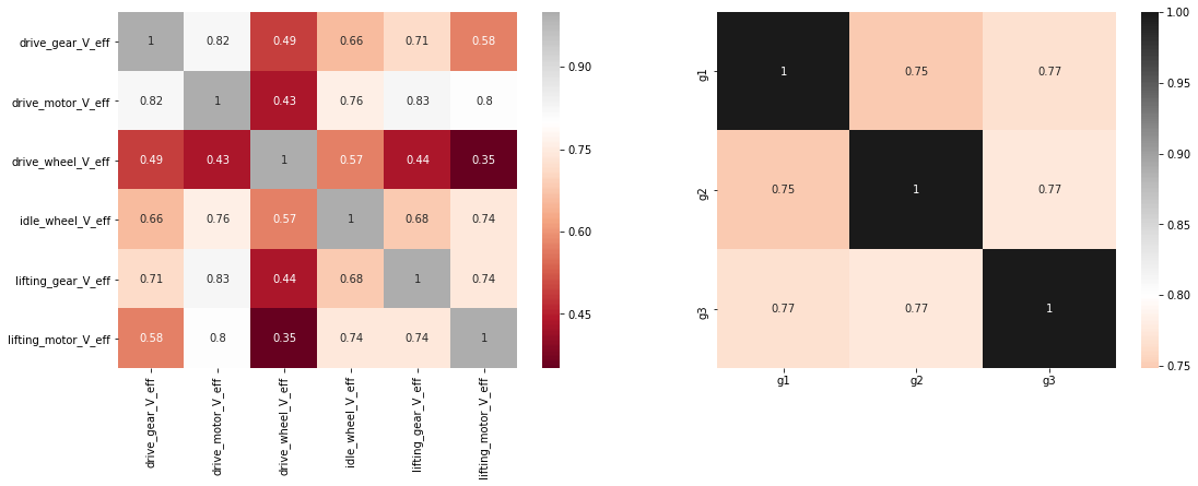
Figure 6: Correlation matrix of sensors from Machine 1. Grey to black indicates high correlation score.
The time series is plotted for each sensors of each machine. No seasonality/repeating patterns/cycles is found. Spectral analysis on Figure 7 confirms the absence of periodicity within the data. This provides a strong case to abandon ARIMA method. At this stage, we consider not using classical time series approaches in favour of Long-Short-Term Memory (LSTM) unit for recurrent neural networks (RNN).

Figure 7: Spectral analysis of Sensor 1 from Machine 1.
Figure 8 shows the plot according to sensor for 7 machines. The patterns in the series suggests that spread may be an indication of the health of the machine. This forms the basis of our study.
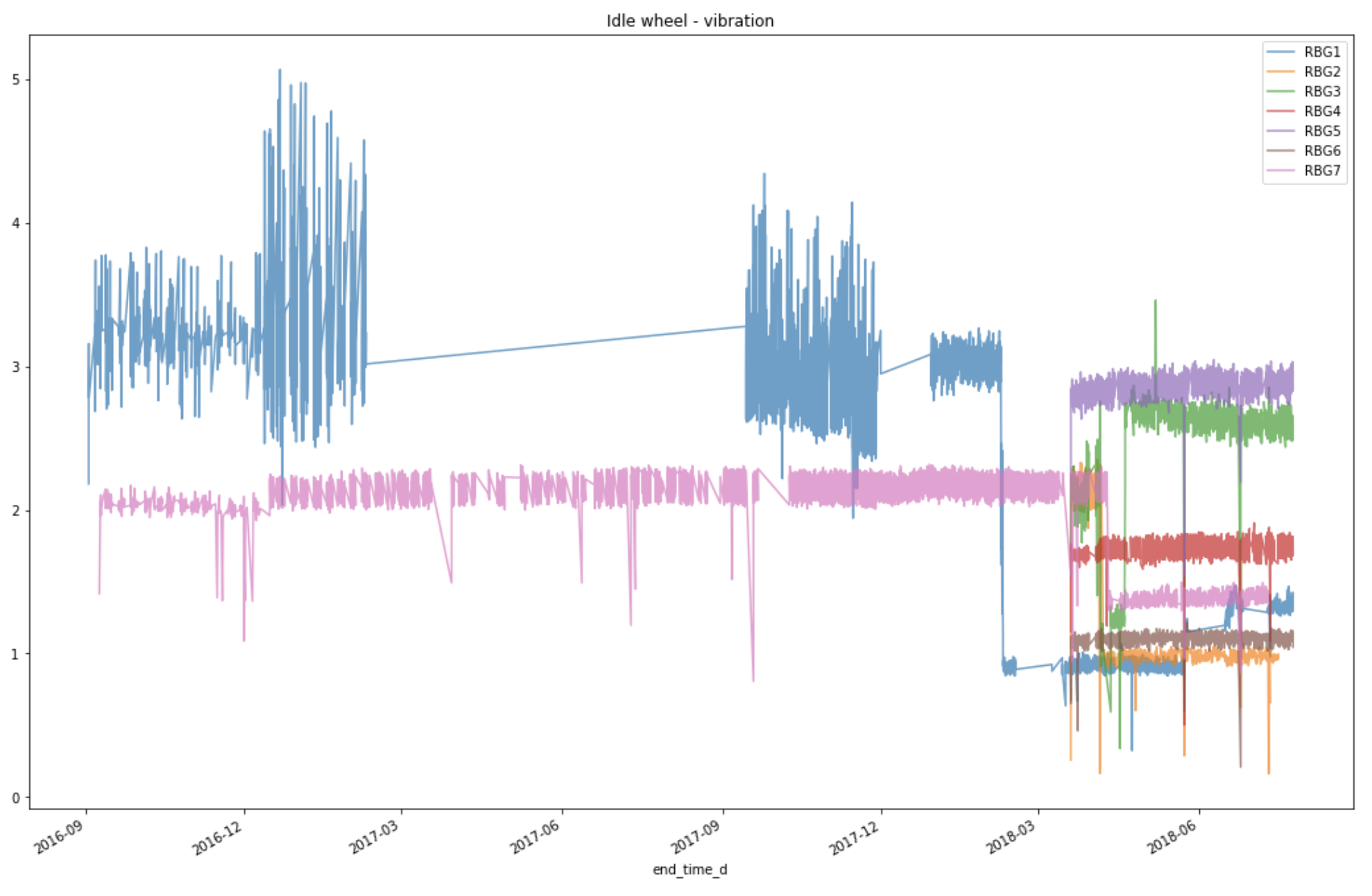
Figure 8: Values of Driver Gear Sensor from 7 machines are plotted at the same axis.
Extreme values in the data are filtered using Tukey’s method. Figure 9 illustrates the occurrence rate of outliers that are present in the sensor data aggregated by machine and sensor type. Visual inspection indicates that Machine 7 shows a significantly higher occurrence of outliers, followed closely by Machines 2 and 3. Interpreting the occurrence of outliers as an indicator of machine reliability, we hypothesize that machine health for Machines 1, 4, 5, and 6 were superior to that of the remaining machines during the period of data recorded. We thus propose that a controlled experiment be designed to test said hypothesis and identify supplementary factors that may contribute towards overall machine health.
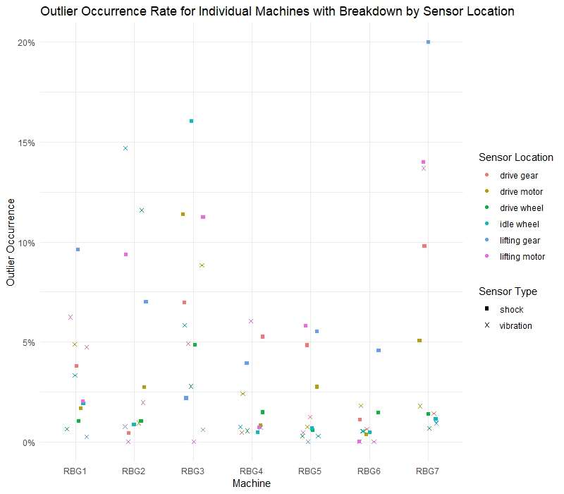
Figure 9: Distribution of outliers
4. Data Preparation
Operations below are performed on the data:
- Datetime variables are converted into machine readable variables.
- Data aggregation is performed to reduce number of rows as well as fill in missing values. Mean is calculated for time interval of 1 minute.
- Some columns are grouped together for exploratory data analysis purpose.
- Outlier removal using standard deviation (Tukey’s Hinges). Any departure from standard operating characteristics are removed.
- Moving variance is calculated with window length of 10 minutes.
5. Modelling and Evaluation
A. AR-LSTM approach
i. Modeling
To detect anomalies in a sensor, we first identify periods for each machine which appear to be well-behaved, fit an AR(10) autoregressive model (10 lags of the variable of interest) after pooling well-behaved series, then forecast the values. If the difference between the forecasted and actual value is ‘high’, the observation will be highlighted as an anomaly.
We begin by modelling the velocity measure, a common parameter for analysing vibration (Scheffer & Girdhar 2004), of the Idle Wheel sensor. This is done by training on data pooled time series data between March 2018 and July 2018, where data is available across all machines. Pooling time series data is not a new idea in the time series literature, although scarcely explored (see Maharaj and Inder 1999). While the functioning of the machine is unknown, the maintenance events (Figure 10) are the next-best option for labelling the data. These models are evaluated by back-casting the series and cross-checking against maintenance events to identify false positives and false negatives.
We consider the use of neural network models for sequence data, particularly recurrent neural network (RNN) models. Traditional RNN units are unable to remember long-term dependencies and susceptible to the vanishing gradient problem, and for this purpose LSTM units may be more suitable.
| machine_name | date | repair_description |
|---|---|---|
| RBG 1 | 13.11.2017 | Correction of skewed movement of the machine on the rail |
| 08.02.2018 | Change of idle wheel | |
| 12.02.2018 – 14.02.2018 | Grinding of the rail | |
| RBG 2 | 02.04.2018 – 08.04.2018 | Grinding of the rail |
| RBG 3 | 02.04.2018 – 08.04.2018 | Grinding of the rail |
| 05.04.2018 | Change of bearings of drive motor | |
| RBG 7 | 02.04. 2018 - 08.04.2018 | Grinding of the rail |
Figure 10: Repair description for maintenance that has occurred.
As each of these series have different centers and spread, we assume that the number of standard deviations away from the mean is similarly distributed and can be ‘learned’ in the same way (Figure 11).
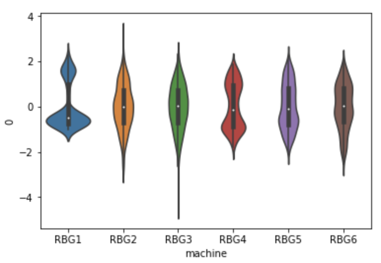
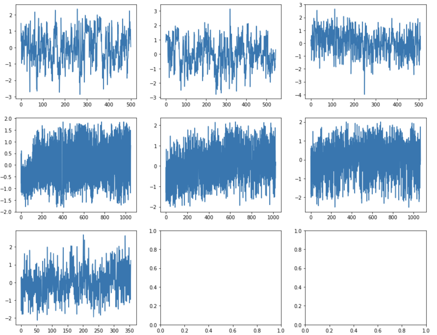
Figure 11: Distribution of Idle Wheel velocity (standardised) across all machines and Time series of each of the machines’ Idle Wheel velocity (standardised)
ii. Evaluation
Evaluation of forecast model
The AR-LSTM model provides forecasts that correspond to the level and spread of data. The spread of the AR-LSTM forecasts (Figure 12) are rather conservative, and the AR-LSTM model performs similarly well out-of-sample.
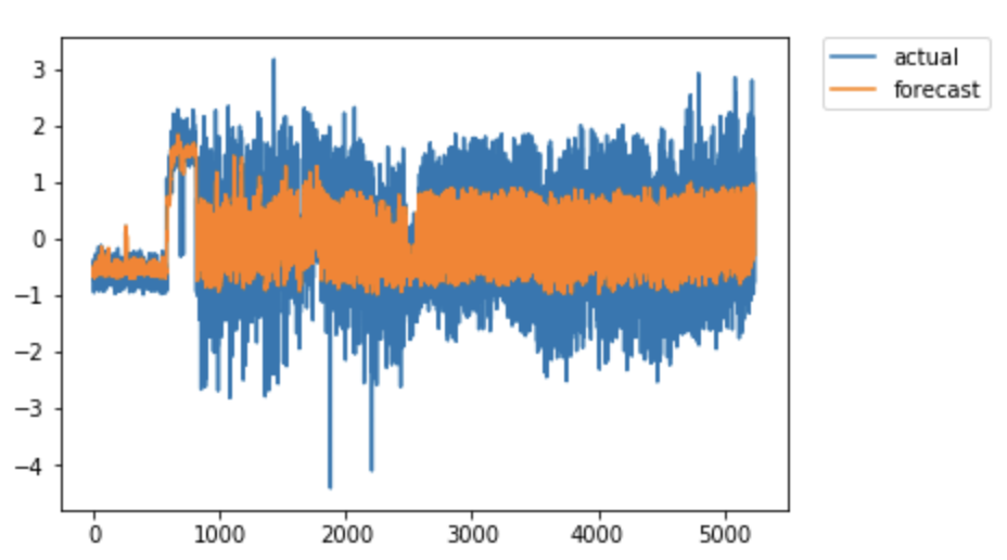
Figure 12: In-sample performance
Evaluation of classification criteria
Figure 13 plots the AR-LSTM forecast errors. We set 3 standard deviations above and below the mean as the threshold for anomalous behaviour. This standard is convenient to interpret as our data is already scaled. This corresponds to approximately 95% of the data, assuming the data is normally distributed. This cut-off rule has a relatively low false positive rate of roughly 18/7000 (0.2%).
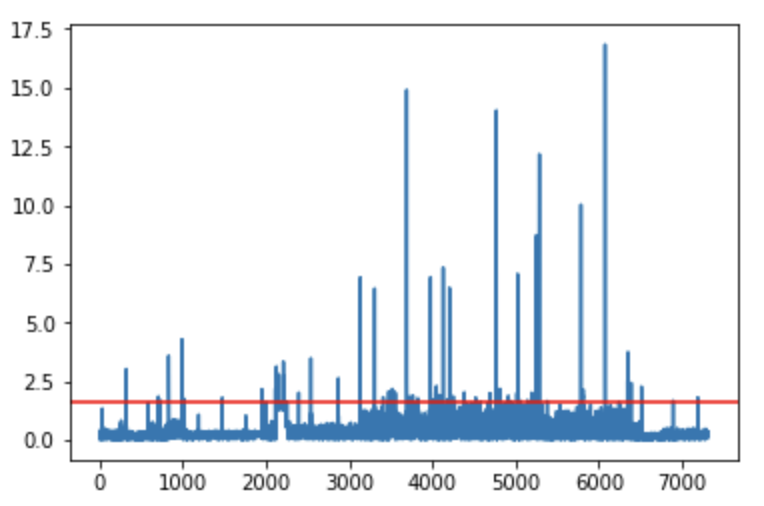
Figure 13: Absolute value of forecast error (standard deviations)
B. Moving variance approach
i. Model
Motivation
We depart from our initial approach of fitting an autoregressive model using LSTM because we cannot easily evaluate our model as the data is unlabelled. Even though a maintenance record is provided, the functioning of the machine remains an unobserved variable. Specifically, we don’t have an idea of machine health, so we can’t evaluate AR-LSTM. Since our EDA suggests we can approximate machine health using the variation in the series, we assume variation to be a general indication of machine health and use LSTM to detect anomalous patterns in the past hour of data.
At a high level, the differences between these two approaches are as follows:
| AR-LSTM | Moving variance approach | |
|---|---|---|
| Predictors | Lagged measure (velocity) | Moving variance of lagged measures |
| Outlier threshold | Standard deviation | Median which is less sensitive to outlier is used |
Figure 15: Major differences in approach
Our use of the spread as a measure of machine health is justified as follows. Figure 16 and 17 show the time series of idle wheel velocity and the moving average respectively, pooled across all machines. It suggests that there are distinct intervals in the data with different spread and centers. This implies that spread may be a good way to indicate machine health.
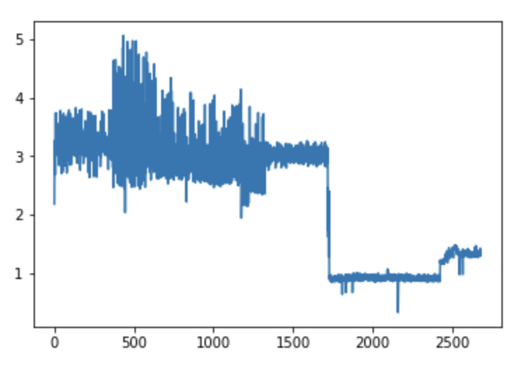
Figure 16: Minute-aggregated time series of idle wheel velocity (machine 1)
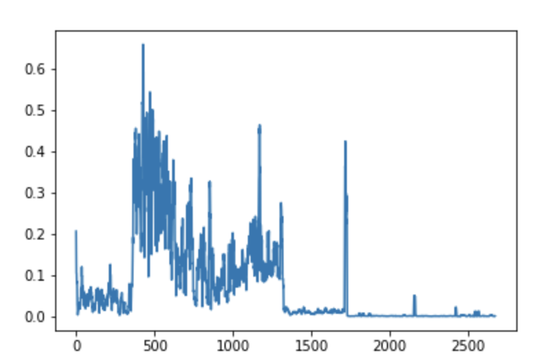
Figure 17: Moving Variance of Idle Wheel velocity (machine 1)
We begin by modelling the velocity measure, a common parameter for analysing vibration (Scheffer & Girdhar 2004), of the Idle Wheel sensor. We generate a series $j$, a pooled time series of velocity for a single sensor $j$ across all machines. Pooling time series data is not a new idea in the time series literature, although scarcely explored (see Maharaj and Inder 1999).
The training set for $v_j$ is generated as a concatenation of velocity data from machines 2 to 7. Data for machine 1 will be used as our test set. Machine 1 is selected because repairs on the idle wheel were only conducted for machine 1.
To use supervised learning methods, we define an anomaly flag, $beta_{j,t}$ to equal True if an observation lies outside of Tukey’s hinges across $v_j$. The anomaly flag is used to flag abnormal behaviour in the sensors. Predictions from the model would indicate that repairs are necessary. In addition, we evaluate the model by back-casting the series. Using the two maintenance events recorded against the idle wheel (Table 1), we can obtain an idea of false positives and false negatives in the data. We emphasise again that we cannot obtain the true rate of false positives and false negatives as machine condition remains latent.
Our exploratory analysis suggests that the variation in the series may indicate the healthy functioning of the machine. We may want to use the instantaneous variation of the series; however the acceleration data does not suggest a relationship between shocks and repair events. As a next-best solution, we use the moving variance to approximate the variation in the series at a point in time.
The moving variance for sensor $j$ across 60 periods, which is equivalent to an hour, is defined as \(s_{j,t}^2=1/60 sumlimits_{i=t-59}^t(v_{j,i}-bar v_{j,t})^2\)
where
\[bar v_{j,t}=1/60 sumlimits_{i=t-59}^t v_{j,i}\]We fit a classification model to classify $beta_{j,t}$ using $s_{j, t-1}, s_{j, t-2},…,s_{j, t-10}$ as predictors. Given that the predictors are sequence data, we consider the use of recurrent neural network (RNN) models for classifying anomalies. Traditional RNN units are unable to remember long-term dependencies and susceptible to the vanishing gradient problem, and for this purpose LSTM units may be more suitable.
We fit two LSTM models for this purpose, with different train/test set pairs (Figure 18). The model summary is shown in Figure 19.
| Train | Test | |
|---|---|---|
| Model 1 | Velocity measure from idle wheel sensors, machines 2 to 7 | Velocity measure from idle wheel sensors, machine 1 |
| Model 2 | Velocity measure from idle wheel sensors, machines 1 to 7 | Velocity measure from lifting motor and drive wheel, machines 1 to 7 |
Figure 18: Train and test set for Models 1 and 2
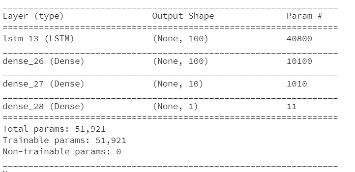
Figure 19: Model summary
ii. Evaluation
Model 1
By visually inspecting Figure 20, observations 300-1300 should be classified as anomalies because the spread of the series is abnormally high. Figure x shows the anomaly flag for Machine 1’s velocity on the idle wheel sensor as classified by Tukey’s method. The anomaly flag correctly highlights these observations as anomalous. The drop-off point at approximately observation 1700 is likely due to a maintenance event. This event is also flagged as anomalous according to Tukey’s Method. Model 1’s predictions also closely follow the anomaly labels.
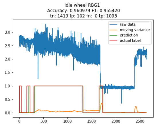
Figure 20: Velocity series of idle wheel for machine 1
Model 2
It is reasonable to assume that the distribution of the normal condition of the sensors is similar across sensors as well as machines. To provide some evidence for our hypothesis, a LSTM model is fitted on the idle wheel data across all machines and tested against lifting motor and drive wheel data across all machines. The results of the predictions on the drive wheel sensors are illustrated in Figure 21.
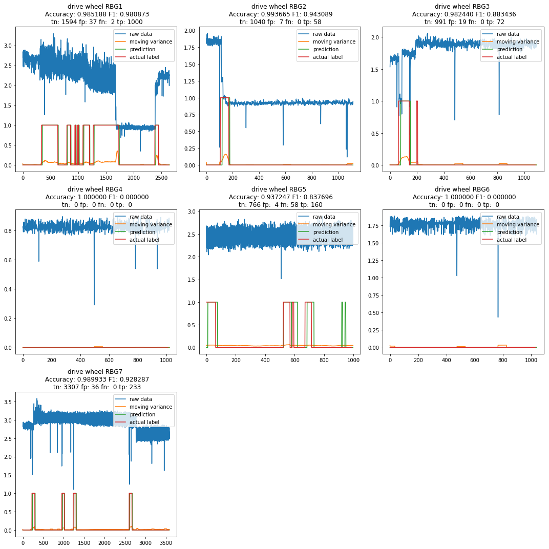
Figure 21: Drive wheel velocity measure for machines 1-7
Again, the predicted data closely trails the actual labels in all drive wheel sensors except for Machine 5, where a false negative was detected. However, the series does not appear to have an abnormal distribution in that region. This suggests that the LSTM approach is able to generalise anomalous patterns better than a naive approach using Tukey’s method to flag anomalies.
As for the lifting motor (Figure 22), the model detects anomalies in Machine 1, 2, 6 and 7. Both the anomaly labels and LSTM predictions detect anomalies similarly. The abnormalities in Machine 1’s idle wheel are reflected in the predictions and anomaly labels for the drive wheel and lifting motor. This suggests that this modelling approach may find it hard to distinguish between different sections of the machine when predicting faults.
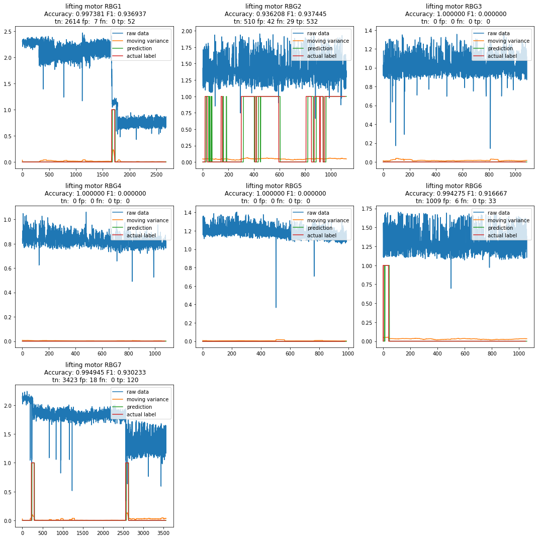
Figure 22: Velocity measures for lifting motor for machines 1-7
Assuming the anomaly labels to be the ‘ground truth’, we can calculate false positive and false negative rates. False negatives are lower than false positives in all sensor-machine combinations evaluated except for Machine 5’s drive wheel sensor. Even though the LSTM model was not optimsed to minimise false negatives, Model 2 has a low share of false negatives.
C. E-Divisive with Medians (EDM)
E-Divisive with Medians (EDM) is a model for breakpoint (changepoint) detection. Breakpoint detection describes the process of detecting change points in time series. We decided to analyse the breakpoints with an unsupervised approach as we noticed that there are visually obvious changes of distribution resulting in distinct segments in the sensor’s time series data, due to different possible reasons (could be anomalies, repairs or maintenances, in some cases it’s missing data). The EDM algorithm (James et al. 2014) is reported to have several advantages over traditional breakout detection techniques. They include (1) robustness against anomalies, (2) able to detect divergence and change in distributions, and (3) faster computation process. In Figure 23, we segment out series into 3 sections by visually examining the data. We expect the EDM algorithm to automate this process.
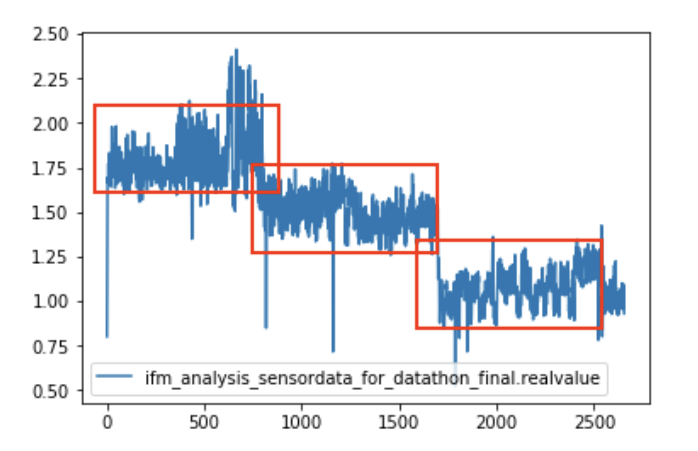
Figure 23: Visual inspection of series
Outcome
We tried to detect the breakouts using different metrics, namely mean (Figure 24), distributions (Figure 25), and median (Figure 26). With no labeled data available, we visually evaluated the graphs and observed that median-based method draws a cleaner boundary between different segments in the time series. We concluded that median is the best option to detect breakouts in our case as it is robust against outliers. One downside of this approach is that computing the median is computationally expensive, with a computational cost of **</b>O(n!)</b>O(n!)</b>O(n!).
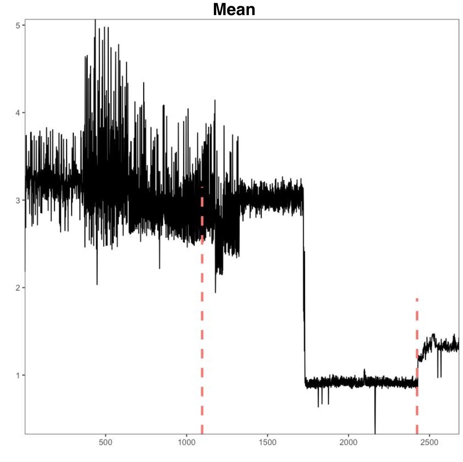
Figure 24: Mean-based EDM
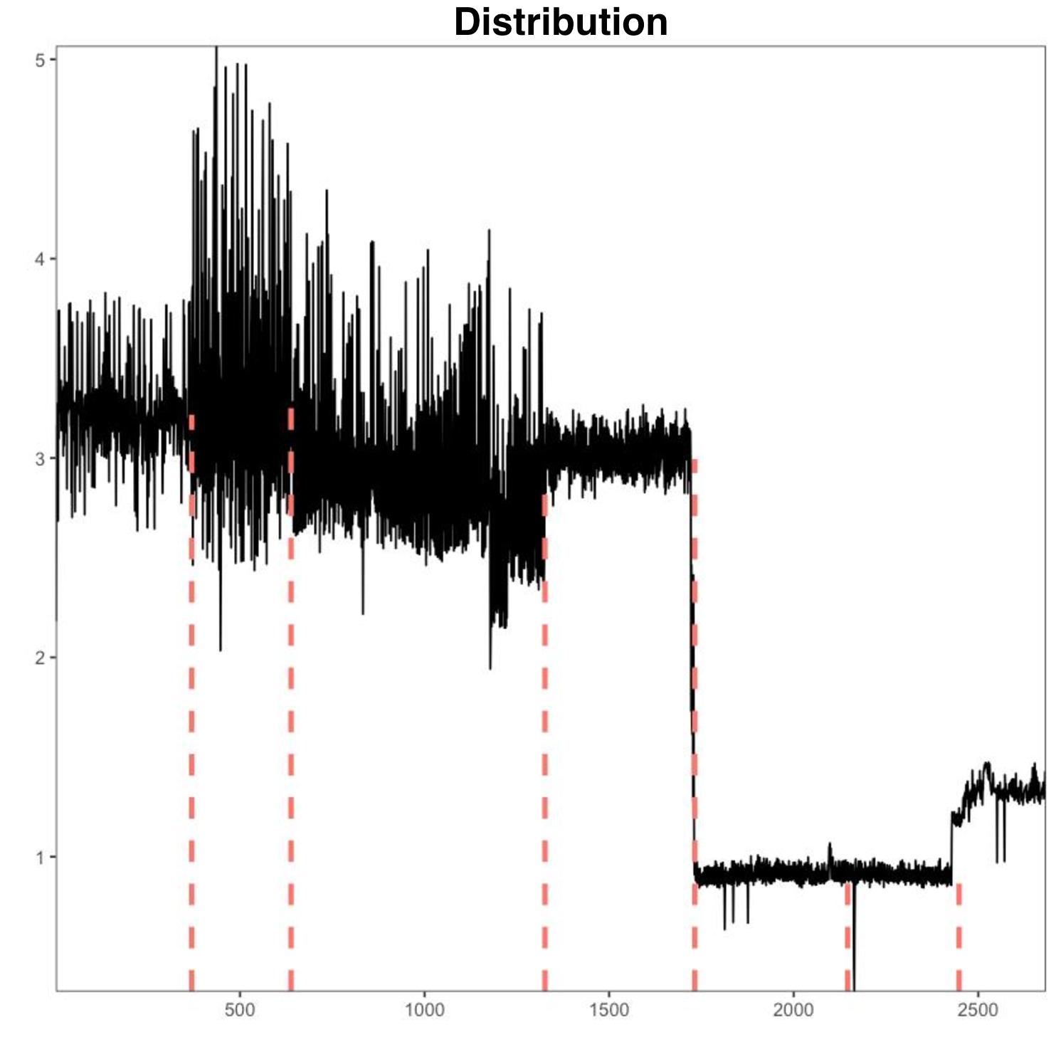
Figure 25: Distribution-based method
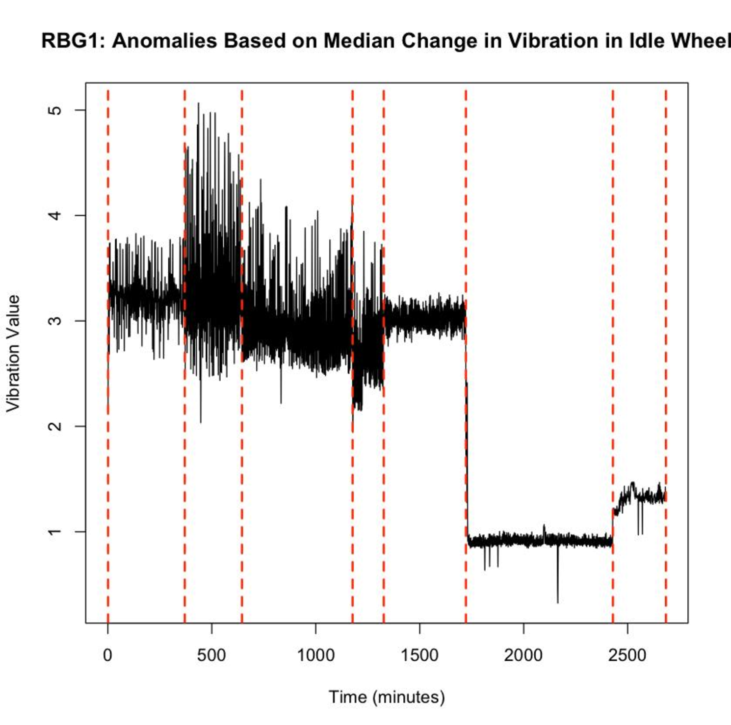
Figure 26: Median-based EDM
Breakpoint detection can indicate gradual shifts in the time series that may not be visible to the human eye. As a complement to actual anomaly detection, it can be deployed to provide alerts before an abrupt anomalous event occurs. This in theory can be used as an indicator for scheduling preventative maintenance.
6. Deployment
A. AR-LSTM
Figure 27 shows the deployment of the AR-LSTM model. Firstly, 11 minutes of data is collected. 10 minutes of data would be sent to LSTM model to make a ‘normal’ prediction, which is the 11th minute. The prediction is then compared to the data collected from the sensor, at the 11th minute since the start.
The difference between the prediction and the real data is calculated. If the difference is greater than the threshold, anomaly is detected since the data deviates from the predicted ‘normal’ value. Otherwise it means there is no anomaly, the machine is operating as normal. The loop continues.
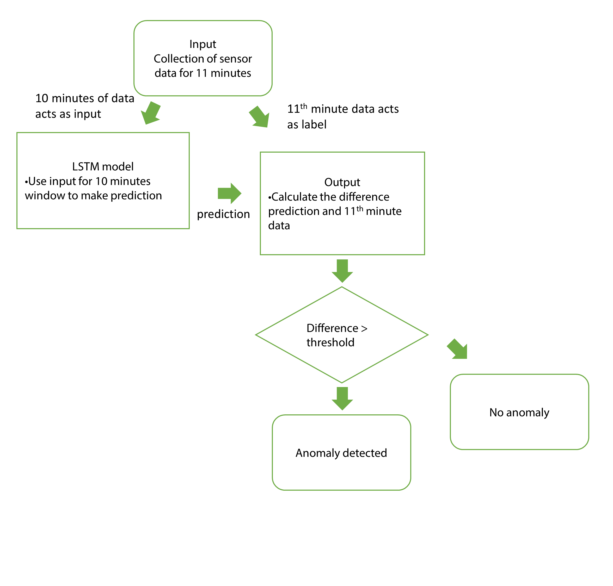
Figure 27: AR-LSTM deployment plan
B. Moving Variance
Figure 28 shows the deployment of the moving variance model. Data is collected for 70 minutes. Data is transformed by computing moving variances for 60 minute windows. Then, predictions are made based on the LSTM model. Based on the prediction, the model suggests whether preventive maintenance is required.
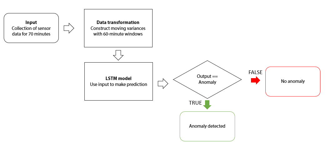
Figure 28: Moving variances-LSTM deployment plan
Conclusion
To sum up our analysis, we have achieved two main actionable outcomes (1) a classification model for outlier detection, and (2) an implementation of breakout detection. With that, we suggest that Kaufland can (1) implement the breakout detection method to alert operators that the machines need to be inspected, (2) use the trained classification model to improve performance of outlier and breakout detection, and finally, (3) do outlier detection in conjunction with detailed repair logs to correlate repair parts with anomalous patterns. In addition, we also recommend several steps that can be taken to improve the overall analyses and modeling: collection of temperature data, machine utilization data, machine movement data and maintaining updated detailed repair logs.
References
- James, N., Kejariwal A.m, and Matteson, D. (2014). Leveraging Cloud Data to Mitigate User Experience from ‘Breaking Bad’. Available at: https://arxiv.org/pdf/1411.7955.pdf
- Girdhar,Paresh dan C. Scheffer., 2004, Practical Machinery Vibration Analysis and Predictive Maintenance., Elsevier, Burlington. Gates corp., 2015.
- Forecasting time series from clusters. Maharaj, E. A. & Inder, B. A. 1999 Melbourne Vic Australia: Monash University Publishing. 27 p.